1. Understanding transformations #
What they handle, where and in which order.
The principle #
Available in: ✓ OSS ✓ Enterprise ✓ Cloud
A transformation changes the result of queries before it is displayed, without touching the data source. Each query returns one or more data frames: tables with fields (columns), a type per field (time, number, string, boolean) and possibly labels. Transformations are chained: each one receives the previous one's output.
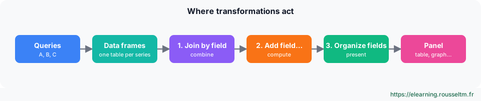
Where are they computed? #
Transformations run in the browser, after the data arrives. Consequences: they do not reduce the load on the data source, they slow down rendering when data is large, and they do not apply to alert rules. For an alert, do the computation in the query or with an expression.
Adding, ordering, scoping to a query #
- In the panel editor, Transformations tab › Add transformation: a search box filters the list by name and category (combine, calculate, reorder, filter…).
- Order matters: a rename placed before a join changes the join field's name. Reorder by drag and drop.
- Each transformation can be limited to some queries (per-query filter option in its settings): handy to clean up only query B.
- The eye icon temporarily disables a transformation, the bin deletes it.
Seeing what happens #
- Table view (toggle at the top of the editor): shows the raw data as a table, whatever the panel type.
- Debug (bug icon on a transformation): shows that transformation's input and output side by side.
- Inspect › Data: the “Apply panel transformations” option downloads the CSV with or without transformations.
Best practice : Open Debug mode for every new transformation: 90% of surprises come from a field that does not have the expected name or type.
2. Organizing and cleaning fields #
Rename, hide, reorder, type, format.
Organize fields by name #
The most used transformation: rename a technical field, hide it (eye icon) or reorder columns by drag and drop. A hidden field remains available to later transformations only if they come before it.
| Before | After |
|---|---|
Value #A, __name__, job, instance | Instance, Requests/s (job and __name__ hidden) |
Rename fields by regex #
Renames several fields at once with a regular expression and capture groups. Example: .*instance="([^"]+)".* replaced with $1 turns {instance="web-1:9100", job="node"} into web-1:9100.
Good to know : For a Prometheus series, the simplest option is often the query Legend ({{instance}}): the name is set at the source.Filter fields by name #
Keeps or removes fields by checkbox or by regular expression (^(Time|instance|Value.*)$). Faster than Organize fields when the query returns many labels.
Convert field type #
Changes a field type: string to number (a CSV or JSON API often returns numbers as text), string to time with a format (YYYY-MM-DD HH:mm:ss), number to boolean, or to Enum. Without the right type, a calculation or time graph fails.
Format string, Format time #
- Format string: upper case, lower case, title case, trimming, substring, to harmonize text values.
- Format time: displays a time field in a chosen format (
DD/MM/YYYY) and time zone, for example in an events table.
3. Filtering, sorting and limiting rows #
Keeping only what matters.
Filter data by values #
Keeps or removes the rows matching conditions on one or more fields: greater, lower, equal, between, regular expression, empty. Conditions are combined with “all” or “any”.
| Condition | Result |
|---|---|
Status matches 5.. (regex) | only server error rows remain |
Usage > 80 and env = prod | saturated production machines |
Filter data by query refId #
Keeps only the results of some queries (A, C…): useful when a query is only used for a calculation or a join and must not be displayed.
Sort by, Limit #
Sort by sorts on a field, ascending or descending; Limit keeps the first N rows. Together they build a “top N”: sort by descending latency then limit to 5.
Best practice : When possible, do the top N in the query (topk(5, …)in PromQL,ORDER BY … LIMIT 5in SQL): the source returns less data.
4. Calculating #
Creating values and summarizing series.
Add field from calculation #
Adds a computed field. The mode determines the calculation:
| Mode | Computation | Example |
|---|---|---|
| Binary operation | two fields or a field and a constant: + − × ÷ % | Used / Total, then × 100 |
| Reduce row | aggregates several fields of the same row: sum, mean, max… | total requests of three services |
| Unary operation | function on one field: absolute value, exponential, logarithm, rounding | abs(Delta) |
| Cumulative functions | running total or mean from the first row | cumulative deployments over the month |
| Window functions | mean, standard deviation or variance over a moving window | 5-point moving average to smooth a curve |
| Row index | row number | rank in a top N |
Give the new field an alias and tick “Replace all fields” if only the result should remain.
Reduce #
Summarizes each series into one or more statistics (last non-null value, mean, max, min, total, count…). Two modes:
- Series to rows: one row per series, one column per statistic. Ideal for a summary table (one row per server with Mean, Max, Last).
- Reduce fields: keeps the structure but reduces each field to one value; “Labels to fields” option keeps labels as columns.
| Before (3 time series) | After Reduce › Series to rows (Mean, Max) |
|---|---|
| web-1, web-2, web-3 : CPU % every 15 s | web-1 | 34 | 81 web-2 | 28 | 66 web-3 | 52 | 97 |
Regression analysis #
Computes a trend line (or polynomial) from a series and extends it: useful to estimate when a disk will be full. Use with care: a linear trend ignores cycles and clean-ups.
5. Combining several queries #
Join, merge, concatenate.
Join by field #
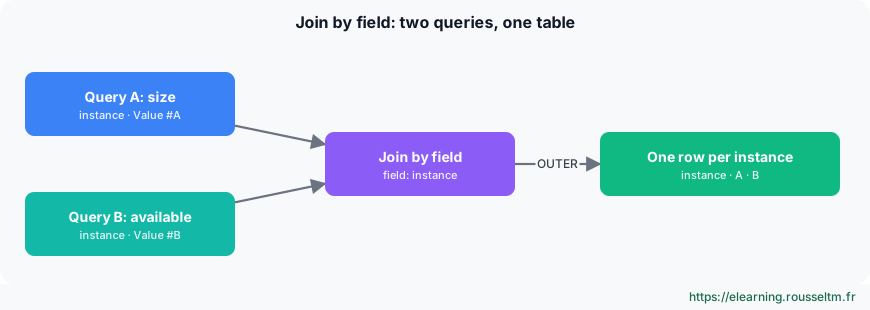
Joins data frames on a common field (time by default, or a field such as instance). Modes:
| Mode | Keeps |
|---|---|
| OUTER (time series) | every time value from both sides; empty cells when a series has no point |
| OUTER (tabular) | every row, for non-time tables |
| INNER | only values present on both sides |
| LEFT | every row of the first query, completed by the second |
Watch out : Both join fields must have exactly the same name and type. Rename before the join, and for Prometheus use instant queries in Table format.
Join by labels #
Assembles series sharing labels (for example instance and job) into one table where each series becomes a column: handy to put several metrics of the same target side by side.
Merge series/tables #
Merges results with the same structure into one table, aligning fields with the same name: for example three SQL queries on three regional databases, or several Elasticsearch indices.
Concatenate fields, Series to rows #
- Concatenate fields: puts every field of every query side by side, without a join key (rows are aligned by position).
- Series to rows: stacks several time series into one long table (Time, Metric, Value), for an events table or an export.
6. Reshaping data #
From labels to columns, rows to fields, one format to another.
Labels to fields #
Turns series labels into columns (Columns mode) or rows (Rows mode). It is the key to inventory tables built from info metrics such as node_uname_info or kube_pod_info.
| Before | After Labels to fields |
|---|---|
node_uname_info{instance="web-1", release="6.8.0", nodename="web-1"} = 1 | columns instance | release | nodename | Value |
Partition by values #
The opposite of a merge: splits one table into several series by the values of a field. An SQL query returning time, region, sales becomes one line per region, without writing one query per region.
Rows to fields, Grouping to matrix, Transpose #
- Rows to fields: each row becomes a field (the name from one column, the value from another); ideal to show key/value pairs in a Stat panel.
- Grouping to matrix: cross table, one field as rows, another as columns, a value in the cells (hour × day, service × environment).
- Transpose: swaps the rows and columns of a table.
Prepare time series, Time series to table #
- Prepare time series: converts data between multi-frame, wide (one time column, several value columns) and long (time, label, value) formats, so a time series panel accepts it.
- Time series to table: puts a small sparkline of each series in a table cell.
Extract fields, Config from query results #
- Extract fields: extracts fields from a JSON, key=value or delimited column (Loki logs, API responses), with selected JSON paths.
- Config from query results: uses a query result as a setting (threshold, min, max, unit) for the others: the threshold comes from a reference table instead of being typed in.
7. Grouping and aggregating #
The GROUP BY equivalent.
Group by #
Groups rows by one or more fields (Group by) and aggregates the others (Calculate: sum, mean, count, last value…).
| Before: one row per container | After Group by host, Count |
|---|---|
| host | container | memory web-1 | api | 512 web-1 | nginx | 64 web-2 | api | 498 | host | containers | memory (sum) web-1 | 2 | 576 web-2 | 1 | 498 |
Group to nested tables, Histogram #
- Group to nested tables: one row per group, expandable to show the group's rows in a nested table.
- Histogram: computes the distribution of values into buckets, for example the spread of response times over the period.
8. Complete recipes #
Ready-to-reproduce transformation chains.
Disk usage per server #
Two instant Prometheus queries, Table format:
A: node_filesystem_size_bytes{fstype!~"tmpfs|overlay", mountpoint="/"}
B: node_filesystem_avail_bytes{fstype!~"tmpfs|overlay", mountpoint="/"}- Join by field on
instance(OUTER tabular mode). - Add field from calculation, Binary operation:
Value #B / Value #A, aliasFree; then a second one:1 - Free, aliasUsage, unit Percent (0.0-1.0). - Organize fields by name: keep
instanceandUsage, rename. - Sort by
Usagedescending; thresholds at 80% and 90% in the panel.
Good to know : Same result directly in PromQL: 1 - node_filesystem_avail_bytes / node_filesystem_size_bytes. The recipe remains useful when both values come from different sources.Server inventory #
node_uname_info- Instant query in Table format.
- Labels to fields (if the source returns series) then Filter fields by name:
instance,nodename,release,machine. - Organize fields by name to rename (Server, Kernel, Architecture) and Sort by Server.
Top 5 slowest routes #
histogram_quantile(0.95, sum by (le, route) (rate(http_request_duration_seconds_bucket[5m])))- Instant query, Table format; Organize fields by name:
routeand the value renamedp95. - Sort by
p95descending, then Limit to 5. - Add field from calculation, Row index, alias
Rank.
9. Best practices, alternatives and exercise #
When to transform, when not to.
Query, transformation or SQL expression? #
| Need | Best place |
|---|---|
| aggregate, filter, compute on one source | the query (PromQL, LogQL, SQL) |
| combine different sources, computation also used by an alert | SQL expressions (Grafana 12+, server side) |
| formatting: rename, hide, type, sort an already small result | transformations |
-- SQL expression (Grafana 12+): A and B are the panel's queries
SELECT A.service, A.value AS requests, B.value AS errors,
       ROUND(100.0 * B.value / A.value, 2) AS error_rate
FROM A JOIN B ON A.service = B.service
ORDER BY error_rate DESC
Best practices #
- Reduce data at the source: a transformation over 50,000 rows freezes the browser.
- Name computed fields (alias): later transformations and overrides refer to them by name.
- Keep chains short and readable; beyond six or seven transformations, the query or an SQL expression is often clearer.
- Transformations are part of the panel JSON: they are versioned with Git Sync or provisioning, and kept by Grafana 13's dashboard schema v2.
Cheat sheet #
| I want to… | Transformation |
|---|---|
| rename, hide, reorder | Organize fields by name |
| rename many series | Rename fields by regex |
| change a type (string → number or time) | Convert field type |
| filter rows | Filter data by values |
| a top N | Sort by + Limit |
| a calculation between columns | Add field from calculation |
| one value per series | Reduce |
| combine two queries | Join by field |
| merge identical results | Merge series/tables |
| labels as columns | Labels to fields |
| one series per field value | Partition by values |
| count or sum per group | Group by |
| a cross table | Grouping to matrix |
| read JSON in a column | Extract fields |
Your turn #
- With the TestData data source (“Random walk” scenario, 3 series), build a table with one row per series showing Mean, Max and Last (Reduce › Series to rows).
- Add a
Spreadfield = Max − Mean and sort by spread descending. - Keep only the series whose mean is above 0 (Filter data by values) and rename the columns.
- Open Debug mode on each step and note what changes between input and output.
